multi-area-model
A large-scale spiking model of the vision-related areas of macaque cortex.
This project is maintained by INM-6
Multi-scale spiking network model of macaque visual cortex
![]()

![]()
This code implements the spiking network model of macaque visual cortex developed at the Institute of Neuroscience and Medicine (INM-6), Research Center Jülich. The model has been documented in the following publications:
-
Schmidt M, Bakker R, Hilgetag CC, Diesmann M & van Albada SJ Multi-scale account of the network structure of macaque visual cortex Brain Structure and Function (2018), 223: 1409 https://doi.org/10.1007/s00429-017-1554-4
-
Schuecker J, Schmidt M, van Albada SJ, Diesmann M & Helias M (2017) Fundamental Activity Constraints Lead to Specific Interpretations of the Connectome. PLOS Computational Biology, 13(2): e1005179. https://doi.org/10.1371/journal.pcbi.1005179
-
Schmidt M, Bakker R, Shen K, Bezgin B, Diesmann M & van Albada SJ (2018) A multi-scale layer-resolved spiking network model of resting-state dynamics in macaque cortex. PLOS Computational Biology, 14(9): e1006359. https://doi.org/10.1371/journal.pcbi.1006359
The code in this repository is self-contained and allows one to reproduce the results of all three papers.
A video providing a brief introduction to the model and the code in this repository can be found here.
Try it on EBRAINS
Want to start using or simply run the model? Click the button below.
Please note: make sure you check and follow our User instructions, especially if you plan to make and save the changes, or if you simply need step-by-step instructions.

User instructions
The Jupyter Notebook multi-area-model.ipynb illustrates the simulation workflow with a down-scaled version of the multi-area model. This notebook can be explored and executed online in the Jupyter Lab provided by EBRAINS without the need to install any software yourself.
- Prerequisites: an EBRAINS account. If you don’t have it yet, register at register page. Please note: registering an EBRAINS account requires an institutional email.
- If you plan to only run the model, instead of making and saving changes you made, go to Try it on EBRAINS; Should you want to adjust the parameters, save the changes you made, go to Fork the repository and save your changes.
Try it on EBRAINS
- Click Try it on EBRAINS. If any error or unexpected happens during the following process, please close the browser tab and restart the User instruction process again.
- On the
Lab Execution Sitepage, select a computing center from the given list. - If you’re using EBRAINS for the first time, click
Sign in with GenericOAuth2to sign in on EBRAINS. To do this, you need an EBRAINS account. - Once signed in, on the
Server Optionspage, chooseOfficial EBRAINS Docker image 23.06 for Collaboratory.Lab (recommended), and clickstart. - Once succeeded, you’re now at a Jupyter Notebook named
multi-area-model.ipynb. Click the field that displaysPython 3 (ipykernel)in the upper right corner and switch thekerneltoEBRAINS-23.09. - Congratulations! Now you can run the model. Enjoy!
To run the model, click theRunon the title bar and chooseRun All Cells. It takes several minutes until you get all results.
Please note: every time you click theTry it on EBRAINSbutton, the repository is loaded into your home directory on EBRAINS Lab and it overrides your old repository with the same name. Therefore, make sure you follow the Fork the repository and save your changes if you make changes and want to save them.
Fork the repository and save your changes
With limited resources, EBRAINS Lab regularly deletes and cleans data loaded on the server. This means the repository on the EBRAINS Lab will be periodically deleted. To save changes you made, make sure you fork the repository to your own GitHub, then clone it to the EBRAINS Lab, and do git commits and push changes.
- Go to our Multi-area model under INM-6, create a fork by clicking the
Fork. In theOwnerfield, choose your username and clickCreate fork. Copy the address of your fork by clicking onCode,HTTPS, and then the copy icon. - Go to EBRAINS Lab, log in, and select a computing center from the given list.
- In the Jupyter Lab, click on the
Giticon on the left toolbar, clickClone a Repositoryand paste the address of your fork. - Now your forked repository of multi-area model is loaded on the server. Enter the folder
multi-area-modeland open the notebookmulti-area-model.ipynb. - Click the field that displays
Python 3 (ipykernel)in the upper right corner and switch thekerneltoEBRAINS-23.09. - Run the notebook! To run the model, click the
Runon the title bar and chooseRun All Cells. It takes several minutes until you get all results. - You can modify the exposed parameters before running the model. If you want to save the changes you made, press
Control+Son the keyboard, click theGiticon on the most left toolbar, do git commits and push.
To commit, onChangedbar, click the+icon, fill in a comment in theSummary (Control+Enter to commit)at lower left corner and clickCOMMIT.
To push, click thePush committed changesicon at upper left which looks like cloud, you may be asked to enter your username and password (user name is your GitHUb username, password should be Personal access tokens you generated on your GitHub account, make sure you select therepooption when you generate the token), enter them and clickOk. - If you would like to contribute to our model or bring your ideas to us, you’re most welcome to contact us. It’s currently not possible to directly make changes to the original repository, since it is connected to our publications.
Python framework for the multi-area model
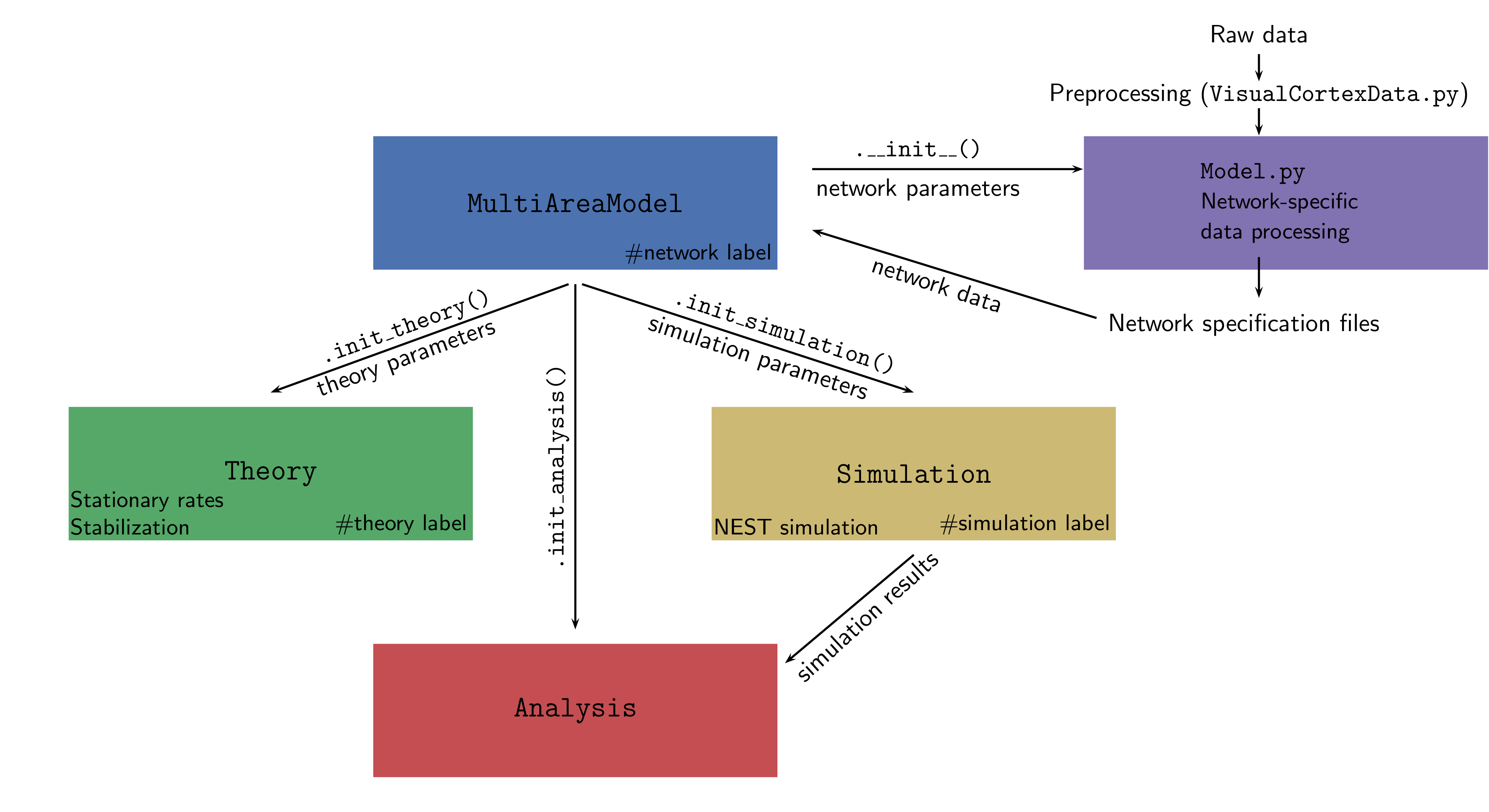
The entire framework is summarized in the figure below:
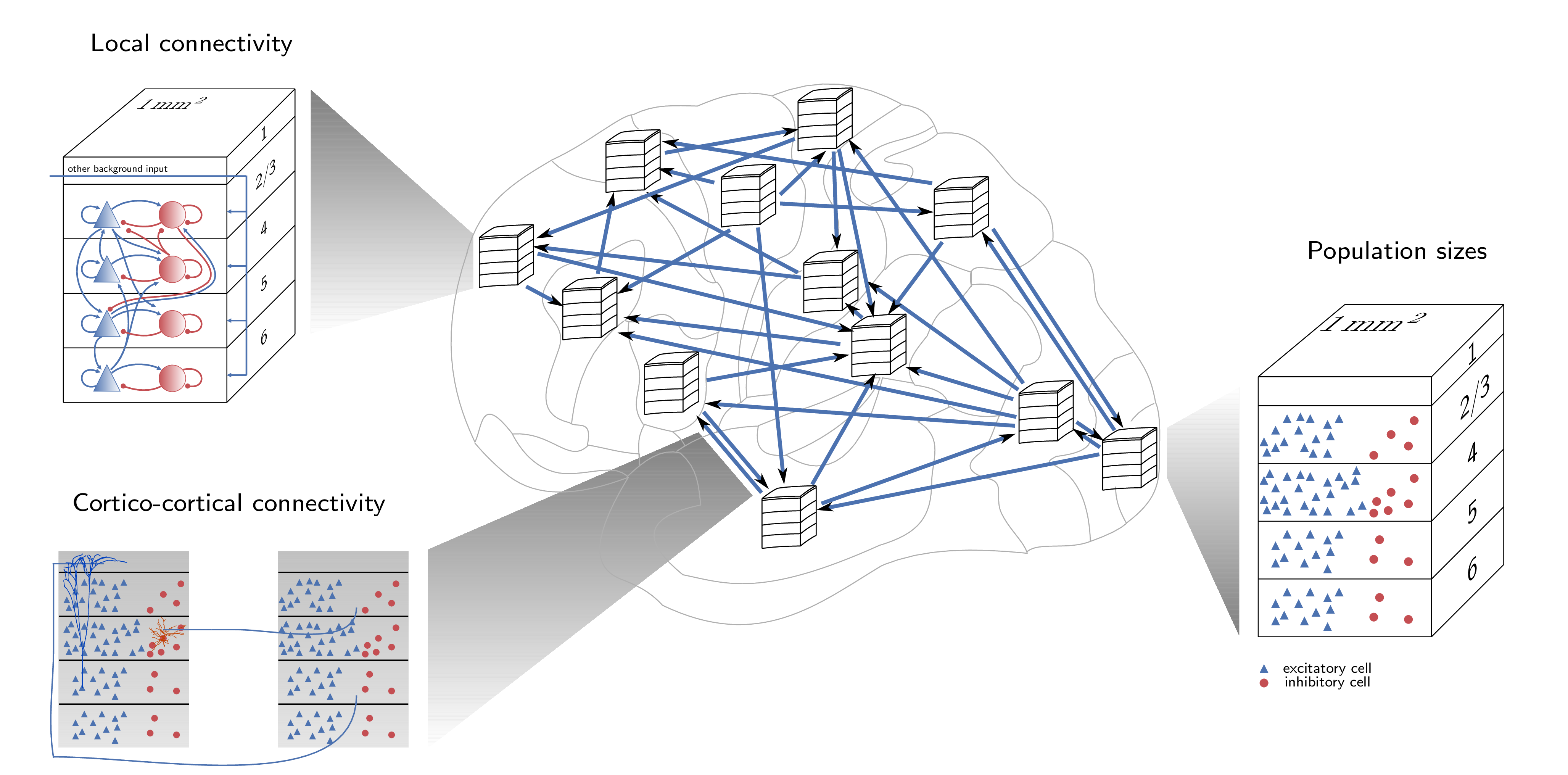
We separate the structure of the network (defined by population sizes,
synapse numbers/indegrees etc.) from its dynamics (neuron model,
neuron parameters, strength of external input, etc.). The complete set
of default parameters for all components of the framework is defined
in multiarea_model/default_params.py.
A description of the requirements for the code can be found at the end of this README.
Preparations
To start using the framework, the user has to define a few environment variables
in a new file called config.py. The file config_template.py lists the required
environment variables that need to be specified by the user.
Furthermore, please add the path to the repository to your PYTHONPATH:
export PYTHONPATH=/path/to/repository/:$PYTHONPATH.
MultiAreaModel
The central class that initializes the network and contains all information about population sizes and network connectivity. This enables reproducing all figures in [1]. Network parameters only refer to the structure of the network and ignore any information on its dynamical simulation or description via analytical theory.
Simulation
This class can be initialized by MultiAreaModel or as standalone and
takes simulation parameters as input. These parameters include, e.g.,
neuron and synapse parameters, the simulated biological time and also
technical parameters such as the number of parallel MPI processes and
threads. The simulation uses the network simulator NEST
(https://www.nest-simulator.org). For the simulations in [2, 3], we
used NEST version 2.8.0. The code in this repository runs with a
later release of NEST, version 2.14.0, as well as NEST 3.0.
Theory
This class can be initialized by MultiAreaModel or as standalone and
takes simulation parameters as input. It provides two main features:
- predict the stable fixed points of the system using mean-field theory and characterize them (for instance by computing the gain matrix).
- via the script
stabilize.py, one can execute the stabilization method described in [2] on a network instance. Please seefigures/SchueckerSchmidt2017/stabilization.pyfor an example of running the stabilization.
Analysis
This class allows the user to load simulation data and perform some basic analysis and plotting.
Analysis and figure scripts for [1-3]
The figures folder contains subfolders with all scripts necessary to produce
the figures from [1-3]. If Snakemake (Köster J & Rahmann S, Bioinformatics (2012) 28(19): 2520-2522)
is installed, the figures can be produced by executing
snakemake in the respective folder, e.g.:
cd figures/Schmidt2018/
snakemake
Note that it can sometimes be necessary to execute snakemake --touch to avoid unnecessary rule executions. See https://snakemake.readthedocs.io/en/stable/snakefiles/rules.html#flag-files for more details.
Running a simulation
The files run_example_downscaled.py and run_example_fullscale.py provide examples. A simple simulation can be run in the following way:
-
Define custom parameters. See
multi_area_model/default_params.pyfor a full list of parameters. All parameters can be customized. -
Instantiate the model class together with a simulation class instance.
M = MultiAreaModel(custom_params, simulation=True, sim_spec=custom_simulation_params) -
Start the simulation.
M.simulation.simulate()
Typically, a simulation of the model will be run in parallel on a compute cluster.
The files start_jobs.py and run_simulation.py provide the necessary framework
for doing this in an automated fashion.
The procedure is similar to a simple simulation:
-
Define custom parameters
-
Instantiate the model class together with a simulation class instance.
M = MultiAreaModel(custom_params, simulation=True, sim_spec=custom_simulation_params) -
Start the simulation. Call
start_jobto create a job file using thejobscript_templatefrom the configuration file and submit it to the queue with the user-definedsubmit_cmd.
Be aware that, depending on the chosen parameters and initial conditions, the network can enter a high-activity state, which slows down the simulation drastically and can cost a significant amount of computing resources.
Extracting connectivity & neuron numbers
First, the model class has to be instantiated:
-
Define custom parameters. See
multi_area_model/default_params.pyfor a full list of parameters. All parameters can be customized. -
Instantiate the model class.
from multiarea_model import MultiAreaModel
M = MultiAreaModel(custom_params)
The connectivity and neuron numbers are stored in the attributes of the model class.
Neuron numbers are stored in M.N as a dictionary (and in M.N_vec as an array),
indegrees in M.K as a dictionary (and in M.K_matrix as an array). To extract e.g.
the neuron numbers into a yaml file execute
   import yaml
   with open('neuron_numbers.yaml', 'w') as f:
       yaml.dump(M.N, f, default_flow_style=False)
Alternatively, you can have a look at the data with print(M.N).
Simulation modes
The multi-area model can be run in different modes.
-
Full model
Simulating the entire networks with all 32 areas with default connectivity as defined in
default_params.py. -
Down-scaled model
Since simulating the entire network with approx. 4.13 million neurons and 24.2 billion synapses require a large amount of resources, the user has the option to scale down the network in terms of neuron numbers and synaptic indegrees (number of synapses per receiving neuron). This can be achieved by setting the parameters
N_scalingandK_scalinginnetwork_paramsto values smaller than 1. In general, this will affect the dynamics of the network. To approximately preserve the population-averaged spike rates, one can specify a set of target rates that is used to scale synaptic weights and apply an additional external DC input. -
Subset of the network
You can choose to simulate a subset of the 32 areas specified by the
areas_simulatedparameter in thesim_params. If a subset of areas is simulated, one has different options for how to replace the rest of the network set by thereplace_non_simulated_areasparameter:hom_poisson_stat: all non-simulated areas are replaced by Poissonian spike trains with the same rate as the stationary background input (rate_extininput_params).het_poisson_stat: all non-simulated areas are replaced by Poissonian spike trains with population-specific stationary rate stored in an external file.current_nonstat: all non-simulated areas are replaced by stepwise constant currents with population-specific, time-varying time series defined in an external file.
-
Cortico-cortical connections replaced
In addition, it is possible to replace the cortico-cortical connections between simulated areas with the options
het_poisson_statorcurrent_nonstat. This mode can be used with the full network of 32 areas or for a subset of them (therefore combining this mode with the previous mode ‘Subset of the network’). -
Dynamical regimes
As described in Schmidt et al. (2018) (https://doi.org/10.1371/journal.pcbi.1006359), the model can be run in two dynamical regimes - the Ground state and the Metastable state. The state is controlled by the value of the
cc_weights_factorandcc_weights_I_factorparameters.
Test suite
The tests/ folder holds a test suite that tests different aspects of
network model initialization and mean-field calculations. It can be
conveniently run by executing pytest in the tests/ folder:
cd tests/
pytest
Requirements
Python 3, python_dicthash (https://github.com/INM-6/python-dicthash), correlation_toolbox (https://github.com/INM-6/correlation-toolbox), pandas, numpy, nested_dict, matplotlib (2.1.2), scipy, pytest, NEST 2.14.0 or NEST 3.0
Optional: seaborn, Sumatra
To install the required packages with pip, execute:
pip install -r requirements.txt
Note that NEST needs to be installed separately, see http://www.nest-simulator.org/installation/.
In addition, reproducing the figures of [1] requires networkx, python-igraph, pycairo and pyx. To install these additional packages, execute:
pip install -r figures/Schmidt2018/additional_requirements.txt
In addition, Figure 7 of [1] requires installing the infomap package to perform the map equation clustering. See http://www.mapequation.org/code.html for all necessary information.
Similarly, reproducing the figures of [3] requires statsmodels, networkx, pyx, python-louvain, which can be installed by executing:
pip install -r figures/Schmidt2018_dyn/additional_requirements.txt
The SLN fit in multiarea_model/data_multiarea/VisualCortex_Data.py and figures/Schmidt2018/Fig5_cc_laminar_pattern.py requires an installation of R and the R library aod (http://cran.r-project.org/package=aod). Without R installation, both scripts will directly use the resulting values of the fit (see Fig. 5 of [1]).
The calculation of BOLD signals from the simulated firing rates for Fig. 8 of [3] requires an installation of R and the R library neuRosim (https://cran.r-project.org/web/packages/neuRosim/index.html).
Contributors
All authors of the publications [1-3] made contributions to the scientific content. The code base was written by Maximilian Schmidt, Jannis Schuecker, and Sacha van Albada with small contributions from Moritz Helias. Testing and review was supported by Alexander van Meegen.
Citation
If you use this code, we ask you to cite the appropriate papers in your publication. For the multi-area model itself, please cite [1] and [3]. If you use the mean-field theory or the stabilization method, please cite [2] in addition. We provide bibtex entries in the file called CITATION.
If you have questions regarding the code or scientific content, please create an issue on github.
![]()
![]()
Acknowledgements
We thank Sarah Beul for discussions on cortical architecture; Kenneth Knoblauch for sharing his R code
for the SLN fit (multiarea_model/data_multiarea/bbalt.R); and Susanne Kunkel for help with creating Fig. 3a of [1] (figures/Schmidt2018/Fig3_syntypes.eps).
This work was supported by the Helmholtz Portfolio Supercomputing and Modeling for the Human Brain (SMHB), the European Union 7th Framework Program (Grant 269921, BrainScaleS and 604102, Human Brain Project, Ramp up phase) and European Unions Horizon 2020 research and innovation program (Grants 720270 and 737691, Human Brain Project, SGA1 and SGA2), the Jülich Aachen Research Alliance (JARA), the Helmholtz young investigator group VH-NG-1028,and the German Research Council (DFG Grants SFB936/A1,Z1 and TRR169/A2) and computing time granted by the JARA-HPC Ver- gabegremium and provided on the JARA-HPC Partition part of the supercomputer JUQUEEN (Jülich Supercomputing Centre 2015) at Forschungszentrum Jülich (VSR Computation Time Grant JINB33), and Priority Program 2041 (SPP 2041) “Computational Connectomics” of the German Research Foundation (DFG).